Sentinel-2 Processing

EOX employs advanced cloud computing and tailored data processing solutions to generate high-quality Earth observation products. By leveraging scalable cloud infrastructure and optimized algorithms, EOX ensures that its datasets are both reliable and consistently processed to meet quality standards. These cloud-native workflows enable rapid data availability, seamless integration with various platforms, and robust handling of large volumes of satellite data, providing users with trustworthy and efficient access to geospatial information.

Search and Metadata Handling

Discovering Sentinel-2 Data via STAC Endpoints

The SpatioTemporal Asset Catalog (STAC) specification enables standardized discovery and access to geospatial data through a JSON-based metadata model. Element84’s EarthSearch API and the Copernicus Data Space STAC Catalogue API both implement this specification, providing programmatic access to Sentinel-2 datasets.

Both APIs support spatial, temporal, and cloud cover filtering and return metadata-rich STAC Items describing Sentinel-2 scenes as well as facilitate scalable, metadata-driven search and retrieval satellite data to support large-scale Earth observation workflows. Their basic features are summarized below:

Feature	EarthSearch (Element84)
Base URL	https://earth-search.aws.element84.com/v1
Data Hosted	Sentinel-2 Level-2A scenes on AWS
Data Format	Cloud-Optimized GeoTIFFs (COGs)
Filtering Options	Spatial bbox/polygon, date range, cloud cover, processing level

Feature	Copernicus Data Space STAC Catalogue
Base URL	https://stac.dataspace.copernicus.eu/v1
Data Hosted	Copernicus Sentinel-2 and other Copernicus products
Data Format	JP2000
Filtering Options	Spatial extent, temporal range, cloud cover, product type

Extracting Angular and Detector Metadata from Sentinel-2 XML

Each Sentinel-2 scene includes a rich metadata package—structured as XML files—containing comprehensive details about the observation. These files follow ESA’s SAFE format and are organized consistently within the product folder structure.

Metadata files provide detailed sensor geometry parameters crucial for directional reflectance modeling:

• Sun Angles: Solar zenith and azimuth angles at acquisition time.
• View Angles: Sensor view zenith and azimuth angles, which vary per detector and across the swath.
• Detector Footprints: Spatial outlines and identifiers of each CCD detector in the MSI instrument array.
• Granule Geometry: Including MGRS granule extents, pixel grid alignment, spatial resolution, and tie point grids.

To utilize these parameters for BRDF correction, the angular data must be extracted and represented on a regular raster grid aligned with the image data. This is typically done by parsing the XML metadata with a custom parser, which navigates the XML tree to retrieve angle arrays and detector geometry.

After parsing, the angular information is transformed into georeferenced raster layers. Using the Mapchete (https://github.com/ungarj/mapchete/) Python library, the angular data arrays can be organized into a Grid geospatial raster like object, which efficiently manages tiled raster grids with spatial referencing. This allows seamless integration of the angular rasters with Sentinel-2 imagery tiles and facilitates subsequent BRDF kernel computations on a per-pixel basis.

By combining precise angular metadata extraction with spatially aligned grids, users can apply robust BRDF normalization models — such as RossThick–LiSparse — that require accurate sun and view angles for each pixel. This step is essential to reduce directional effects and improve reflectance consistency across time and sensor geometries.

BRDF Correction

For the EOxCloudless Sentinel-2 data preprocessing following correction inspired by the Harmonized Landsat and Sentinel-2 (HLS) project.

Bidirectional Reflectance Distribution Function (BRDF) correction is crucial in optical remote sensing to account for the anisotropic nature of surface reflectance caused by varying illumination and viewing geometries. The HLS applies BRDF normalization to enable consistent surface reflectance measurements across time, sensors, and observation conditions. This is particularly important for applications such as vegetation phenology, land cover monitoring, and time-series analysis.

The HLS product uses a kernel-driven BRDF model based on the RossThick–LiSparse-Reciprocal formulation. The surface reflectance R is modeled as a linear combination of three terms:

$$R({\theta }_s,{\theta }_v,\varphi )=f_{iso}+f_{vol}\cdot K_{vol}({\theta }_s,{\theta }_v,\varphi )+f_{geo}\cdot K_{geo}({\theta }_s,{\theta }_v,\varphi )$$

where:

• θₛ: solar zenith angle
• θᵥ: view zenith angle
• ϕ: relative azimuth angle
• f₍iso₎: isotropic (Lambertian) reflectance
• f₍vol₎: volumetric scattering coefficient
• f₍geo₎: geometric-optical scattering coefficient
• K₍vol₎, K₍geo₎: Ross-Thick and Li-Sparse kernels, respectively

Ross-Thick Kernel (Volumetric Scattering)

The Ross-Thick kernel simulates volume scattering from dense vegetation, modeled as:

$$K_{vol}=(\frac{\pi }{2}-\xi )\cos \xi +\sin \xi$$

where ξ is the phase angle derived from the sun-sensor geometry.

MODIS BRDF Parameters per Band

The HLS model uses MODIS-derived BRDF kernel weights for each spectral band, based on the MCD43 global albedo product. These are the average parameters:

Band	Wavelength (nm)	f_iso	f_vol	f_geo
Blue	459–479	0.0774	0.0372	0.0079
Green	545–565	0.1306	0.0580	0.0177
Red	620–670	0.1690	0.0461	0.0225
NIR1	841–876	0.3093	0.1058	0.0437
SWIR1	1628–1652	0.2085	0.0533	0.0279
SWIR2	2105–2155	0.2316	0.0723	0.0211

These coefficients normalize reflectance to a standard geometry (nadir view, 45° solar zenith), reducing angular biases and harmonizing Landsat-8, Landsat-9, and Sentinel-2 reflectance for consistent time series analysis.

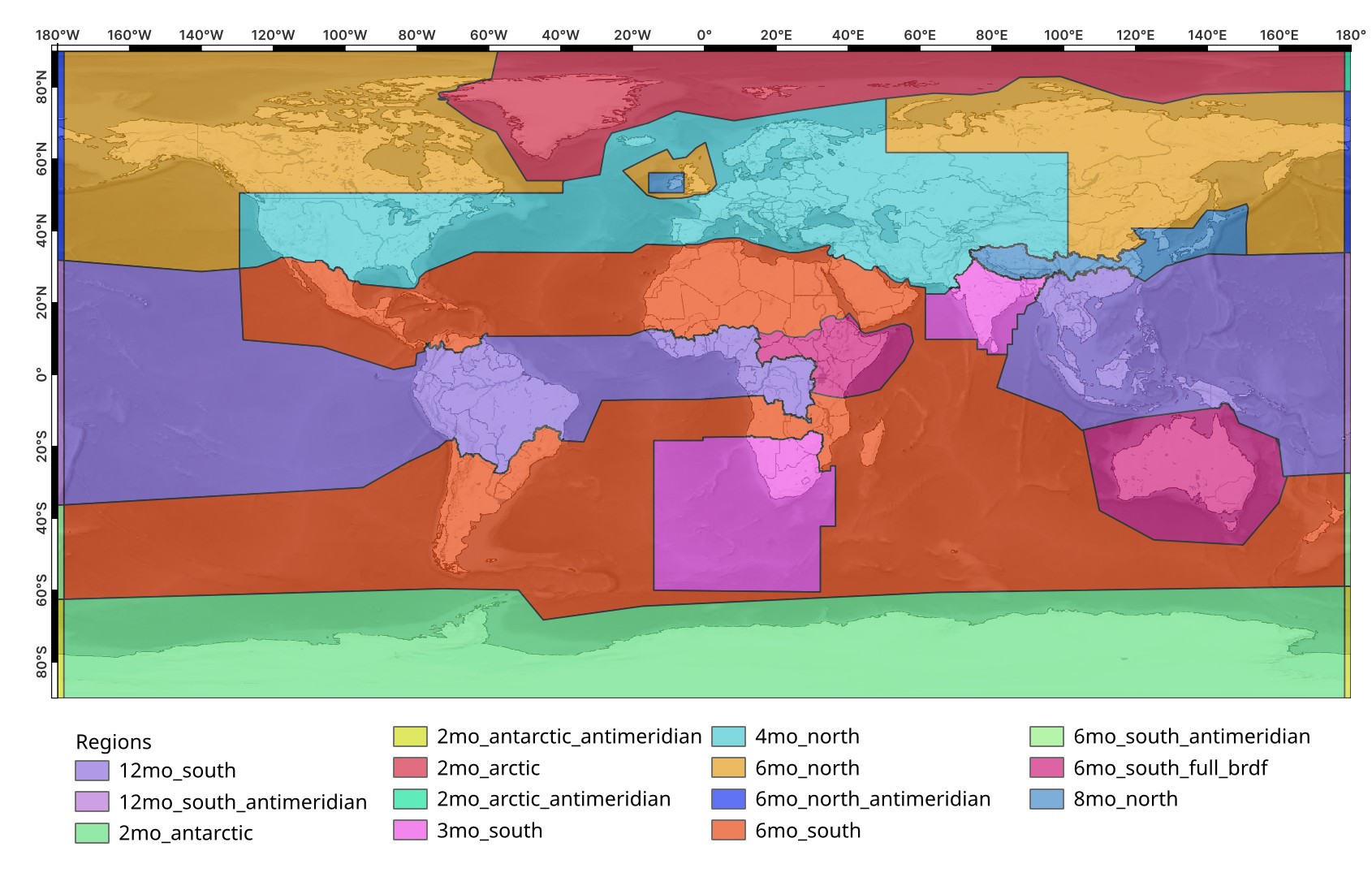
Time Range Selection - Regions

Before diving into the distinct pixel selection that defines the final mosaic, for the annual EOxCloudless product time ranges across the globe need to be taken into consideration as we aim to achieve a "summerlike" mosaic. To achieve this we have split the globe into several regions where we apply different time ranges to focus on the input data time series desired.

Such an approach also allows to utilize multiple search and data source endpoints, in case of inconsistent data over some areas (here around the antimeridian). Additionally, the masks applied and such can also be customized by this approach.

Here is an example of the 2024 EOxCloudless Sentinel-2 regions distribution:

Pixel Selection Methods

Here are the descriptions of the various pixel selection methods provided by the functions:

gap_cluster

The gap_cluster method focuses on extracting pixels by identifying significant "brightness gaps" within the pixel stack. It processes each pixel's temporal data and segments it into clusters based on the two largest brightness differences, effectively separating distinct groups of values. This approach is particularly useful for robustly selecting a representative pixel from an image time series where the "best" pixel might be visually evident by its separation from other values, such as those obscured by clouds or shadows.

jenks_cluster

The jenks_cluster function performs pixel selection by applying the Jenks natural breaks optimization algorithm. This method groups similar pixel values into a specified number of clusters (n_clusters), minimizing the variance within each cluster while maximizing the variance between clusters. Users can then specify a target_cluster to extract values from (e.g., the darkest or a specific brightness range). Further refinement within the target cluster is possible via various option parameters, allowing for the selection of the average, highest saturated pixel, or an average incorporating brightness neighbors.

from_brightness

The from_brightness method selects pixels by first sorting them based on their brightness, primarily determined by the first three bands of the input stack. Once sorted, a specific pixel is chosen according to the extract_method parameter, which can range from statistical measures to extreme values:

• median
• third_quartile
• darkest
• brightest
• second_darkest
• second_brightest

This selection can be further refined by averaging the chosen pixel with its average_over brightness neighbors, providing a smoothed or more representative value.

brightness_sorted

The brightness_sorted method offers a direct way to retrieve the n-th brightest pixel from a given stack. By specifying an index, where 0 represents the darkest pixel, this function sorts the pixels within each stack by their brightness and returns the pixel corresponding to the provided index. This is a straightforward utility for extracting specific brightness quantiles without complex clustering or aggregation.

weighted_avg

The weighted_avg method calculates a biased average from the pixel stack, integrating a sophisticated filtering and weighting scheme. Pixels are filtered using internal cloud and shadow masks and brightness thresholds. Reflectance values are then weighted based on two configurable ranges, enhancing the significance of "optimal" reflectances while reducing the impact of very bright or dark values. The filtered and weighted values are then converted to a logarithmic scale before being averaged, providing a robust mosaic value that prioritizes high-quality observations.

ndvi_linreg

Finally, the ndvi_linreg method leverages linear regression to simulate reflectance values, primarily based on the Normalized Difference Vegetation Index (NDVI) or other indices. It first filters and weights pixel values similarly to weighted_avg to ensure balanced inputs for the linear model. For each band separately, a linear relationship (band value = m*NDVI + n) is derived from the weighted input values. The function then scales the output using a simulation_value for the NDVI, allowing for the generation of synthetic reflectance values. It also includes a fallback mechanism to from_brightness mosaicing if insufficient values are available for the regression.

max_ndvi

The max_ndvi method is designed to identify and extract the "greenest" pixel, resulting in a maximum NDVI mosaic from the input stack. After initial filtering by cloud, shadow, and brightness masks, the function evaluates the NDVI values of the remaining pixels. It then outputs the pixel corresponding to the highest NDVI within user-defined min_ndvi and max_ndvi thresholds. This makes it particularly effective for creating composites that highlight areas of peak vegetation health or presence.